Finite Difference Operator
The computation of gradient magnitude using the finite filters \([1,-1]\) and \([1,-1]^T\) is a method commonly applied in the field of digital image processing to approximate the derivative of a function. This filter is particularly used to estimate the gradient in the horizontal direction of an image. The filter \(G_x\) computes the horizontal gradient \(G_y\) by calculating the difference between adjacent pixels. Similarly, the transpose filter \([1,-1]^T\) computes the vertical gradient \(G_y\) These filters highlight edges and transitions in pixel values, and essential for detecting features in images
Once \(G_x\) and \(G_y\) have been computed, the overall gradient magnitude at each pixels is calculated using the fomula:
$$G = \sqrt{G_x ^2 + G_y ^2}$$
This computed gradient magitude provides a scalar value representing the total rate of change in each pixels. High gradient magnitude indicate potential boundaries betwween different image regions, making this method highly effective for edge detection tasks
The filter result is listed below


Applying tje Derivative of Gaussian(DoG) Filter
The Gaussian kernel is an essential tool for smoothing images.
It helps to reduce noise and detail by averaging out the pixels' values based on their spatial closeness.
To generate a Gaussian kernel, we use the function cv2.getGaussianKernel(),
which creates a one-dimensional Gaussian kernel.
This kernel is then converted to a two-dimensional kernel through an outer product of the 1D kernel with its transpose.
The size and standard deviation of the kernel are set to control the amount and scale of smoothing
To enhance edge detection capabilities, we use the Derivative of Gaussian (DoG) method, which involves convolving the Gaussian kernel with a simple difference operator.
The difference operators, typically in the form of [1, -1] for horizontal and its transpose for vertical directions, are used to calculate the first derivatives of the Gaussian kernel.
This convolution process produces two kernels, one for horizontal and another for vertical edge detection.
These derivative kernels are then used to highlight edges in the image, effectively allowing us to capture significant transitions in intensity.
These are the results in this section:


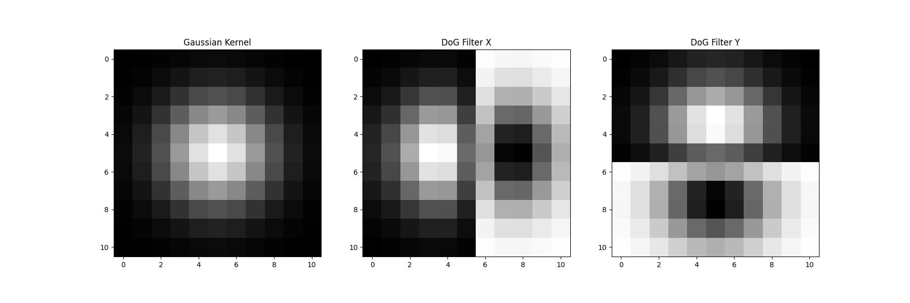
Image Sharpening
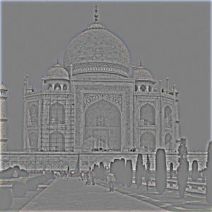
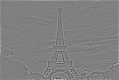
By using Gaussian Filters, the blured images are removed the high frequency values. Using the formula \(high freq = image - blurred image\), we can get high freqency values. Then we add high frequency values on the original image, and we get a sharpen image
Below, you can see a comparison between the original blurred image and the sharpened image. The effects of the technique are visible in the enhanced edges and textures, providing a clearer and more visually appealing result.





Hybrid Images
Hybrid images are constructed by combining the high-frequency component of one image with the low-frequency component of another image. High frequencies are dominant at a closer look but fade away with distance, leaving only the smoother, low-frequency parts visible. This characteristic allows for different interpretations based on viewing distance.
The process involves the following steps:
- Image Selection and Alignment: Choose and align two images to ensure consistent perception grouping.
- Frequency Filtering: Apply a low-pass Gaussian filter to one image to extract its low-frequency components. Subtract this result from the original image to create a high-pass filter output for the second image.
- Image Combination: Combine these two filtered images to create the hybrid image.
To understand the effect of each filtering step, the log magnitude of the Fourier transform is computed for:
- The original images.
- The fft result of each original images.
- The resulting hybrid image.


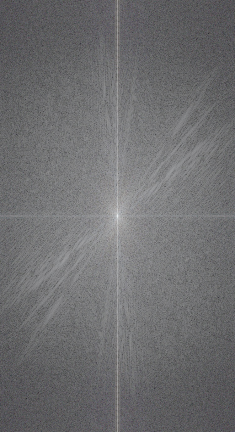
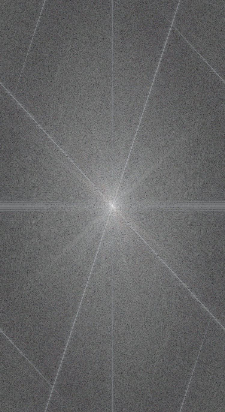
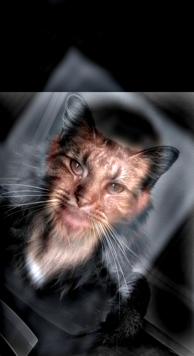
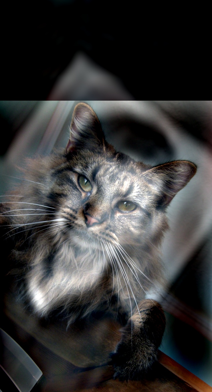
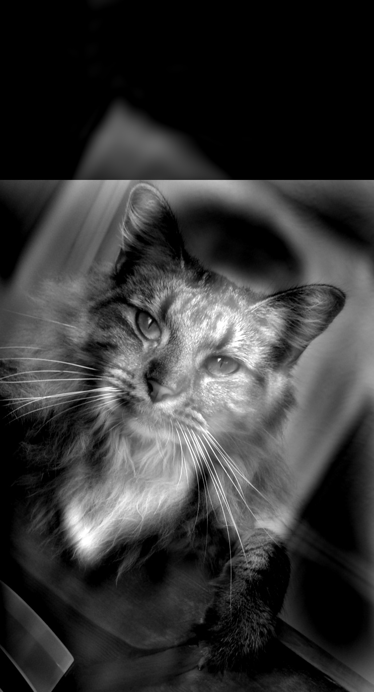


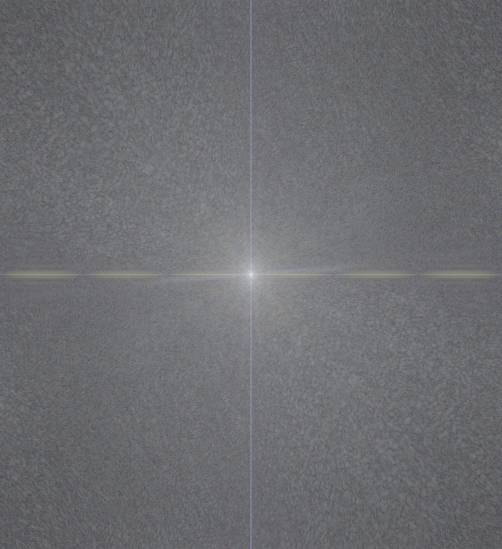

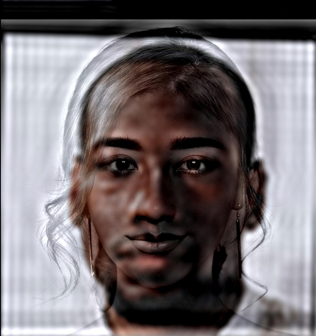
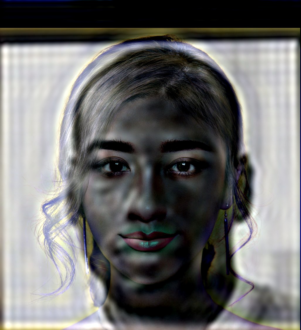
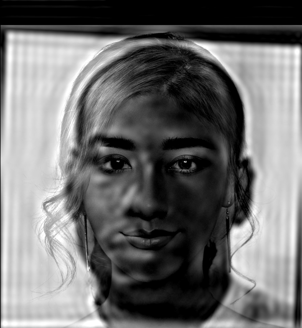
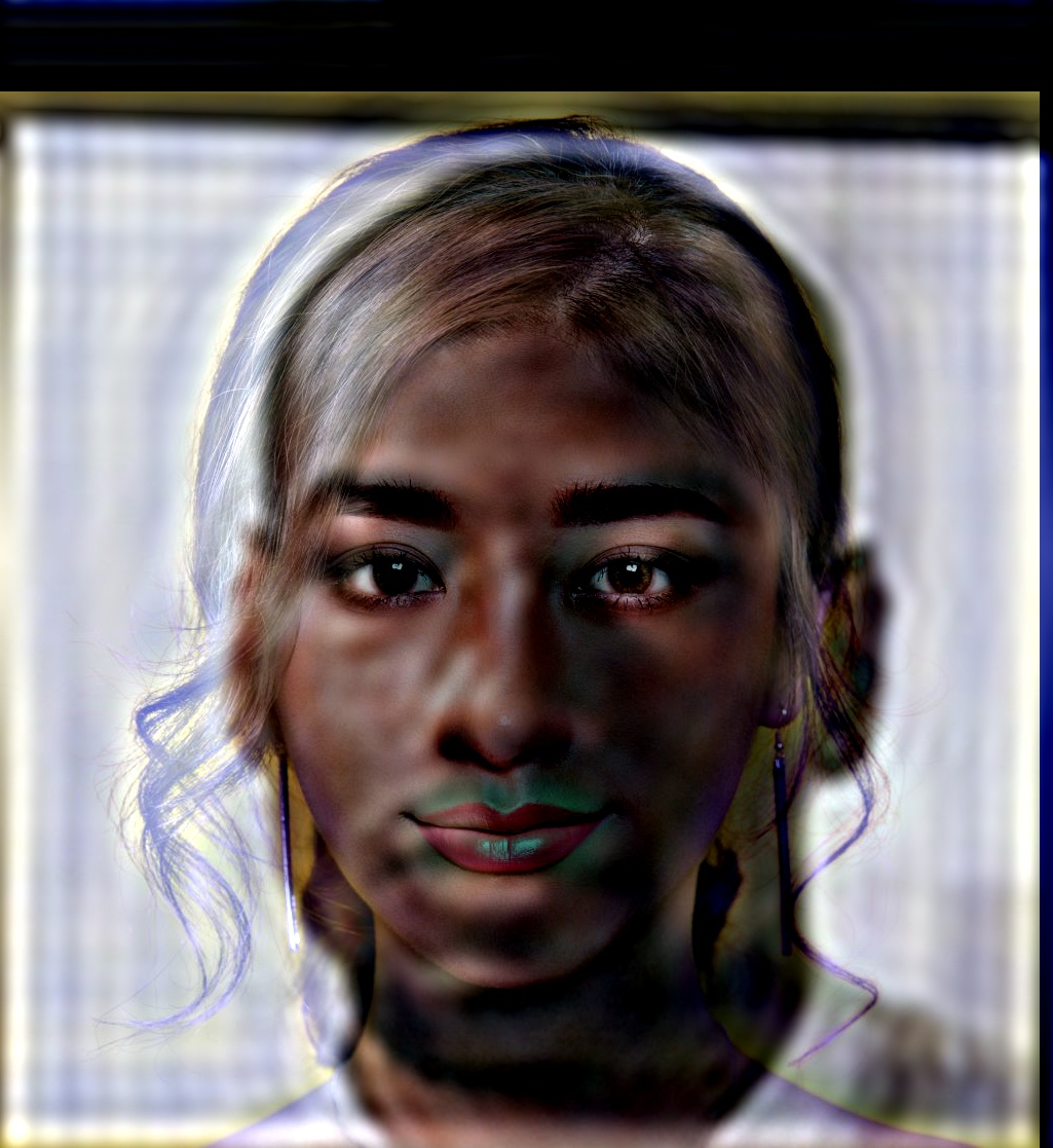
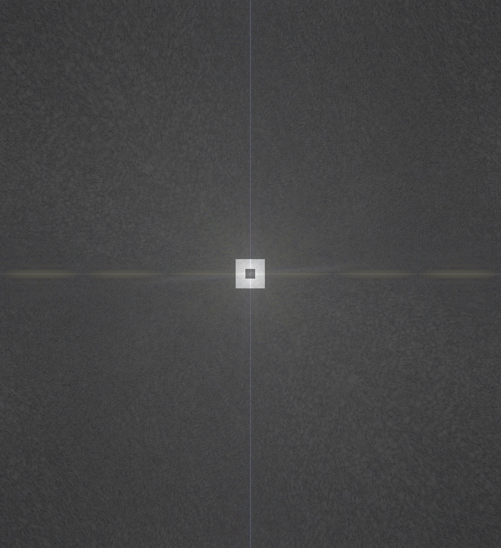


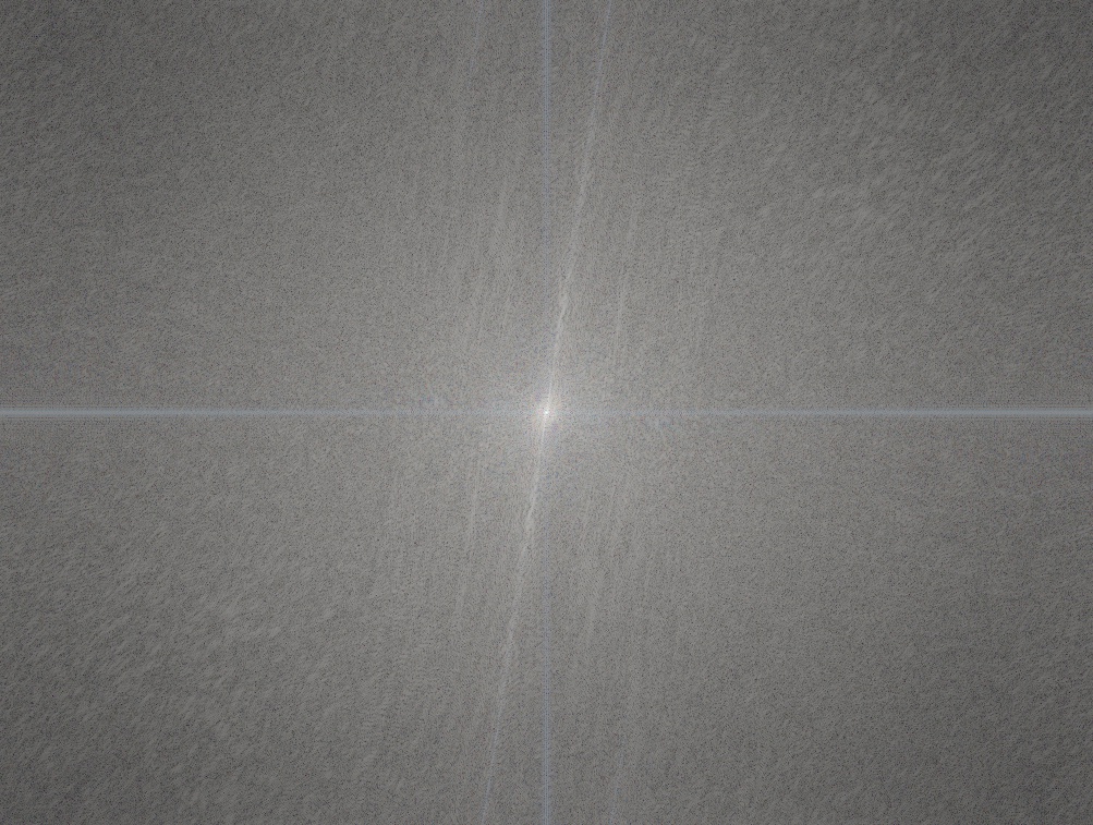
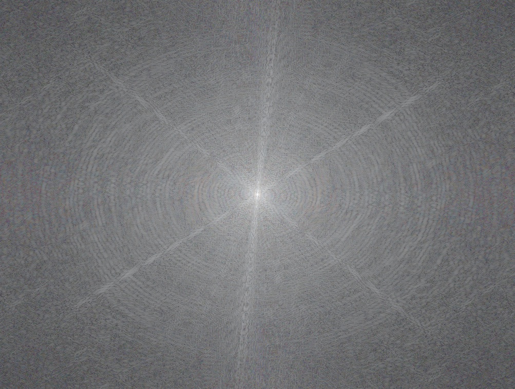


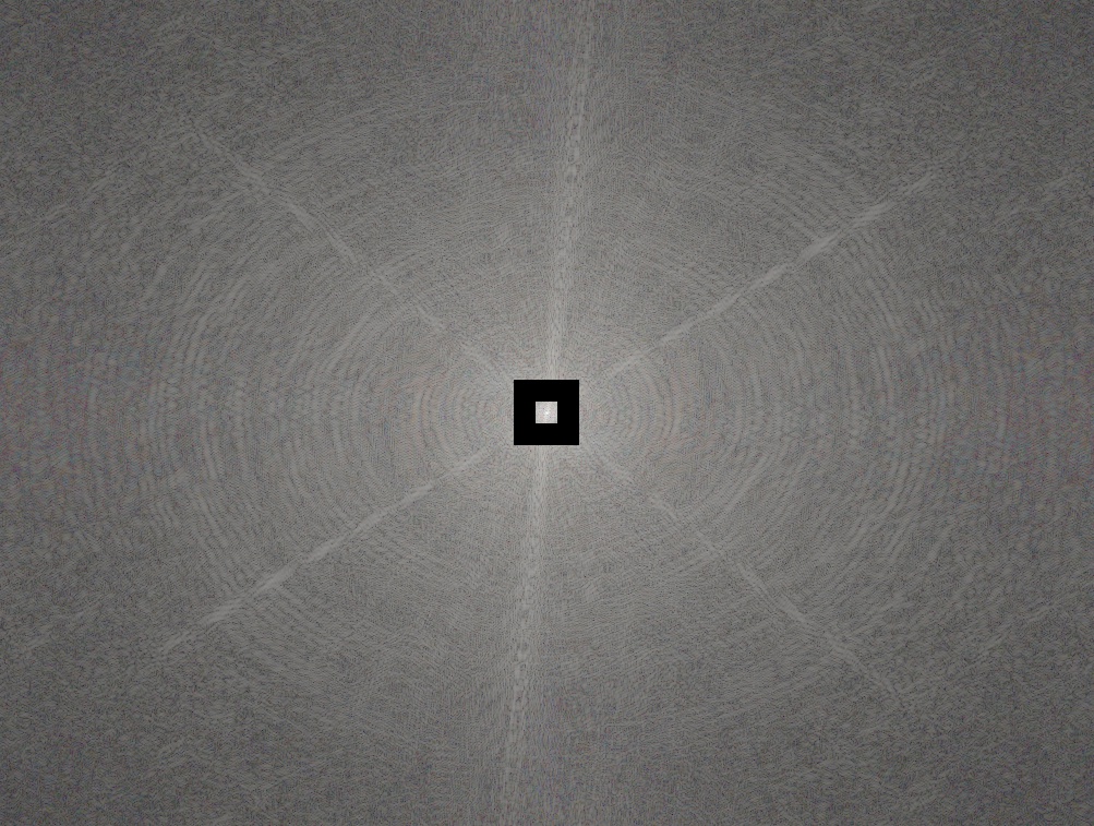
As we can see in the pictures above, the colorful features are mainly existed in low frequecy area, while high frequency area contains information about edges and shape. The reason why my combine fft result have some white or black squares in the center is that I used different cutoff frequency in low and high frequency area, when the frequencies overlap, we will get a black square, else we will get a white one.
Since we have algned two images before hybriding, it's hard to find a proper example for a failure hybrid, because the main objects is finely overlaped and there must have a pair of proper frequencies to seperate them. Based on that, I think it is irreasonable to find a failure example for image hybrid
Multi-resolution Blending and the Oraple journey
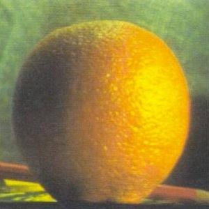
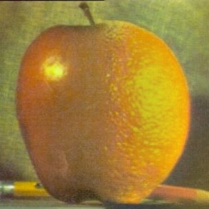
The multi-resolution blending technique, also known as pyramid blending, leverages the power of image pyramids to create seamless blends between two images. This method is particularly effective when combining images with differing characteristics, such as color intensity and structural details, allowing for a smooth transition across the blend.
The Gaussian stack and Laplacian stack of one blending example is listed below


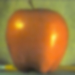


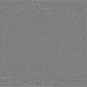
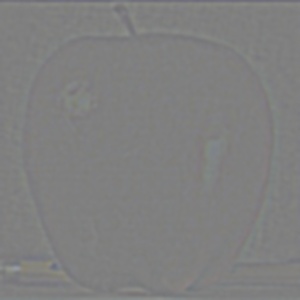
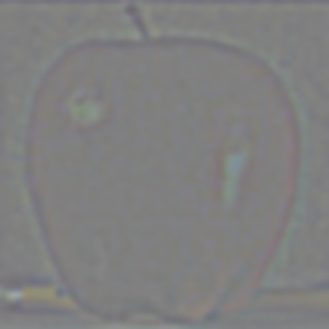


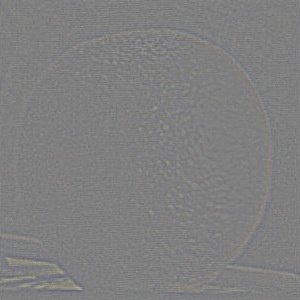


Not only the basic apple and orange blend but also exploring more complex scenarios with irregular blending masks. The results illustrate how different layers of image pyramids interact to synthesize a cohesive final image, adapting to the contours and unique features of each input.
Multi-resolution blending involves the following steps:
- Image Decomposition: Each image is decomposed into a set of multi-scale image pyramids.
- Layered Blending: Corresponding layers of the image pyramids are blended using a mask that defines which parts of each image should appear in the final blend.
- Image Reconstruction: The blended layers are then combined to reconstruct the final image, ensuring that transitions between different resolutions are smooth and natural.
These steps allow for a dynamic blending process that can handle complex image features and varying textures, making it ideal for creating novel visual effects.
Beyond the classical apple and orange combination, our experiments included blends using irregular masks and images with distinct textural differences. These experiments highlight the versatility of multi-resolution blending:
