Project 4
Take Photos
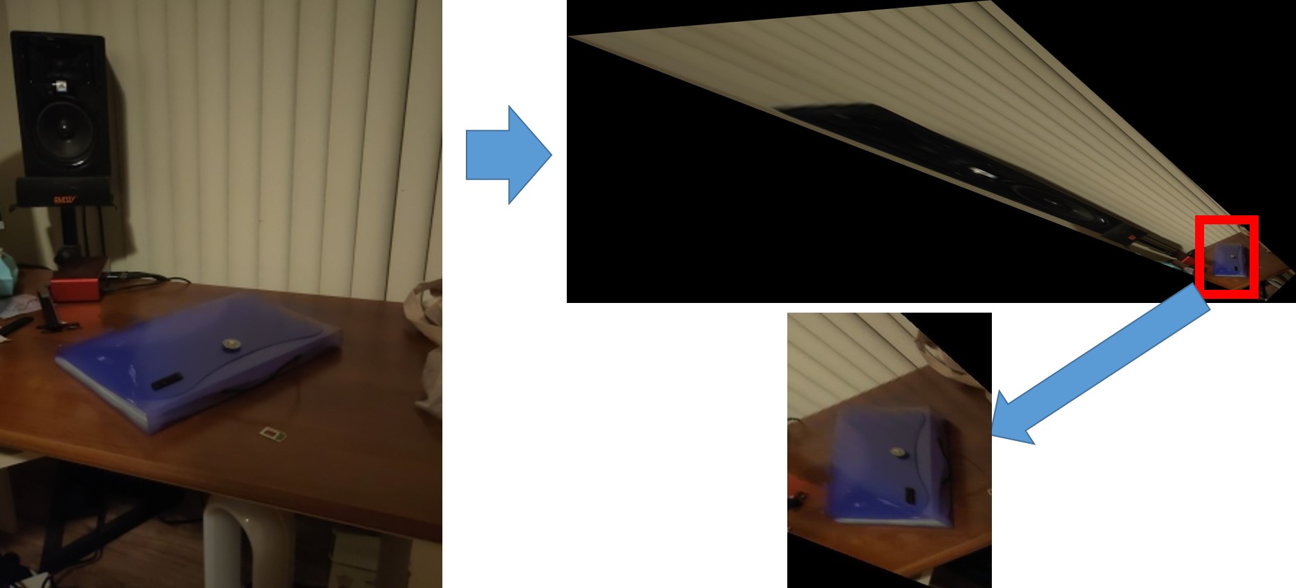
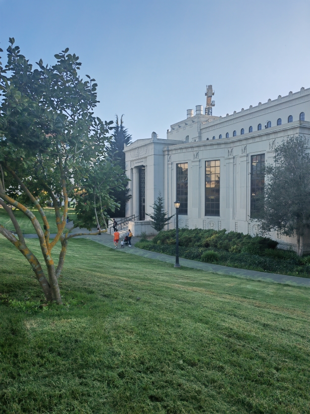
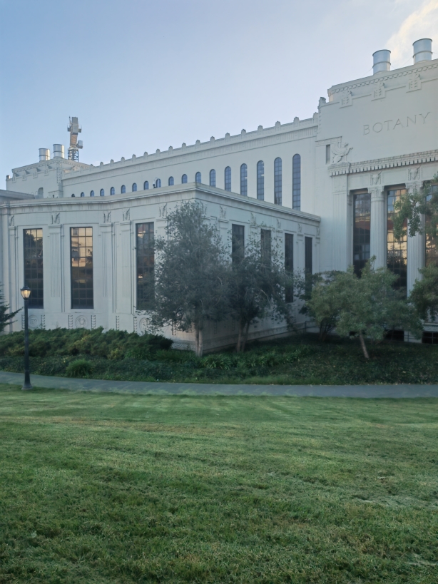
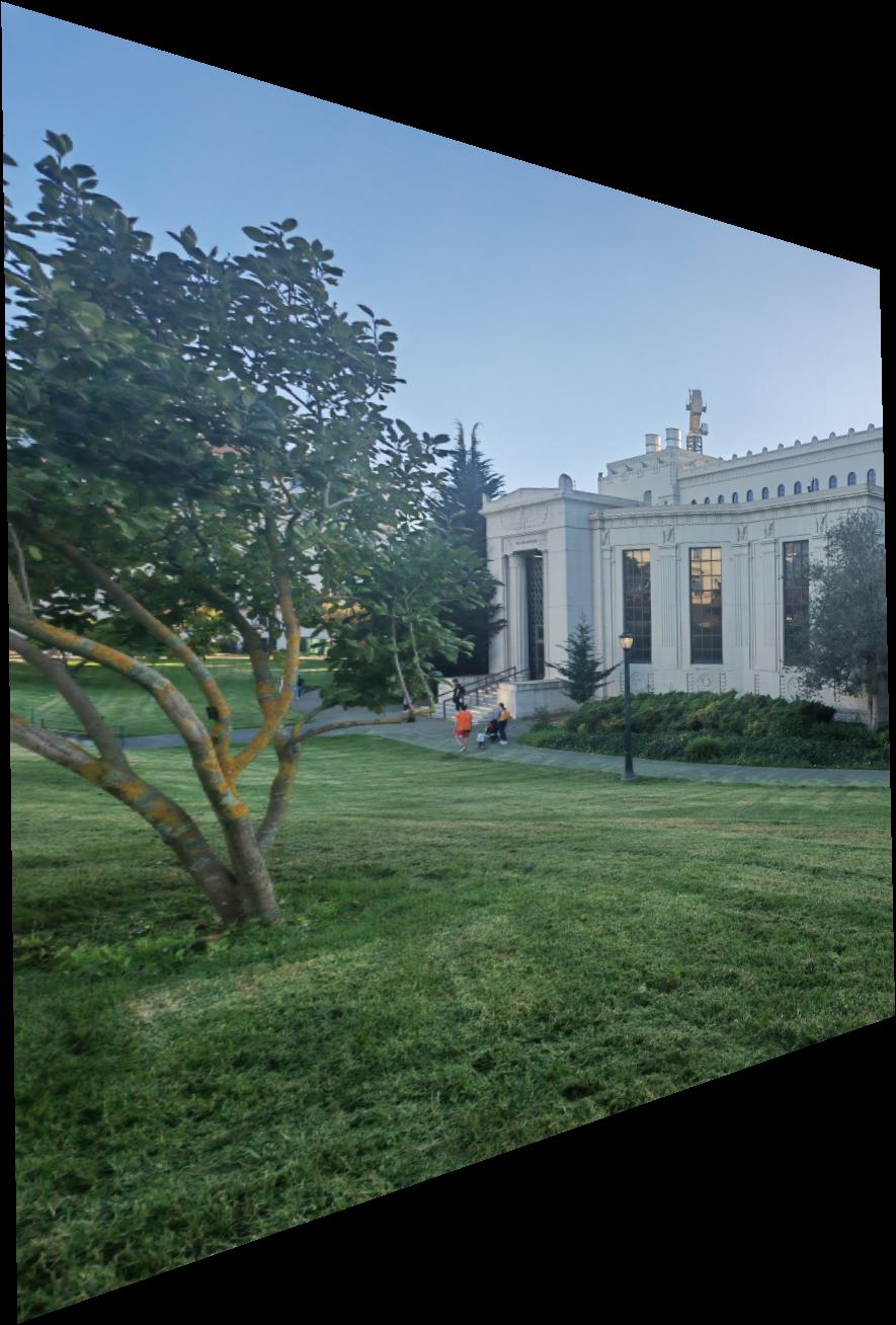
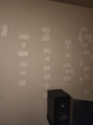
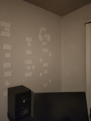
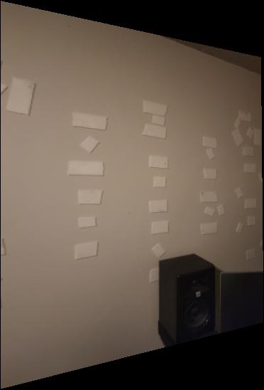
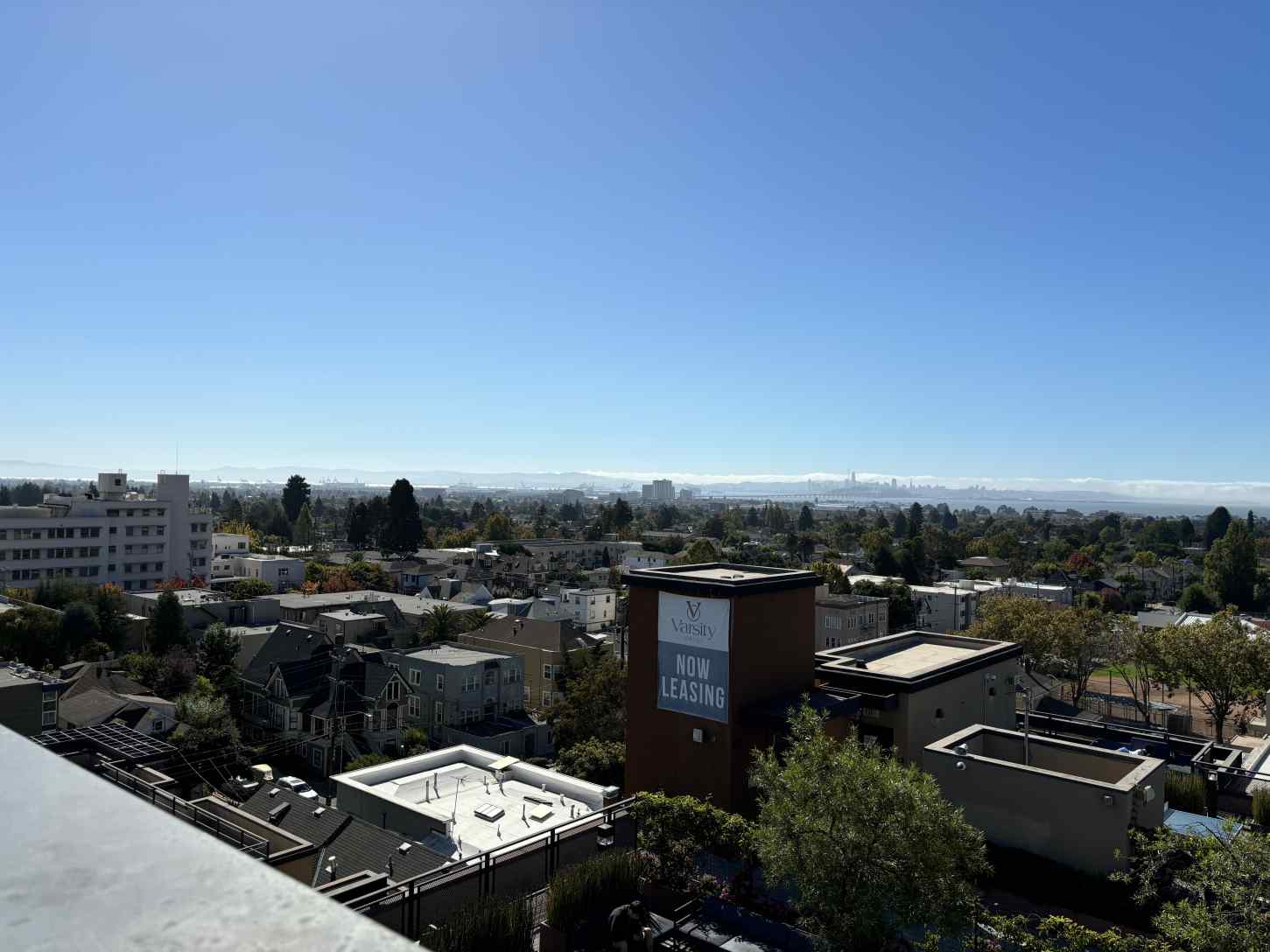
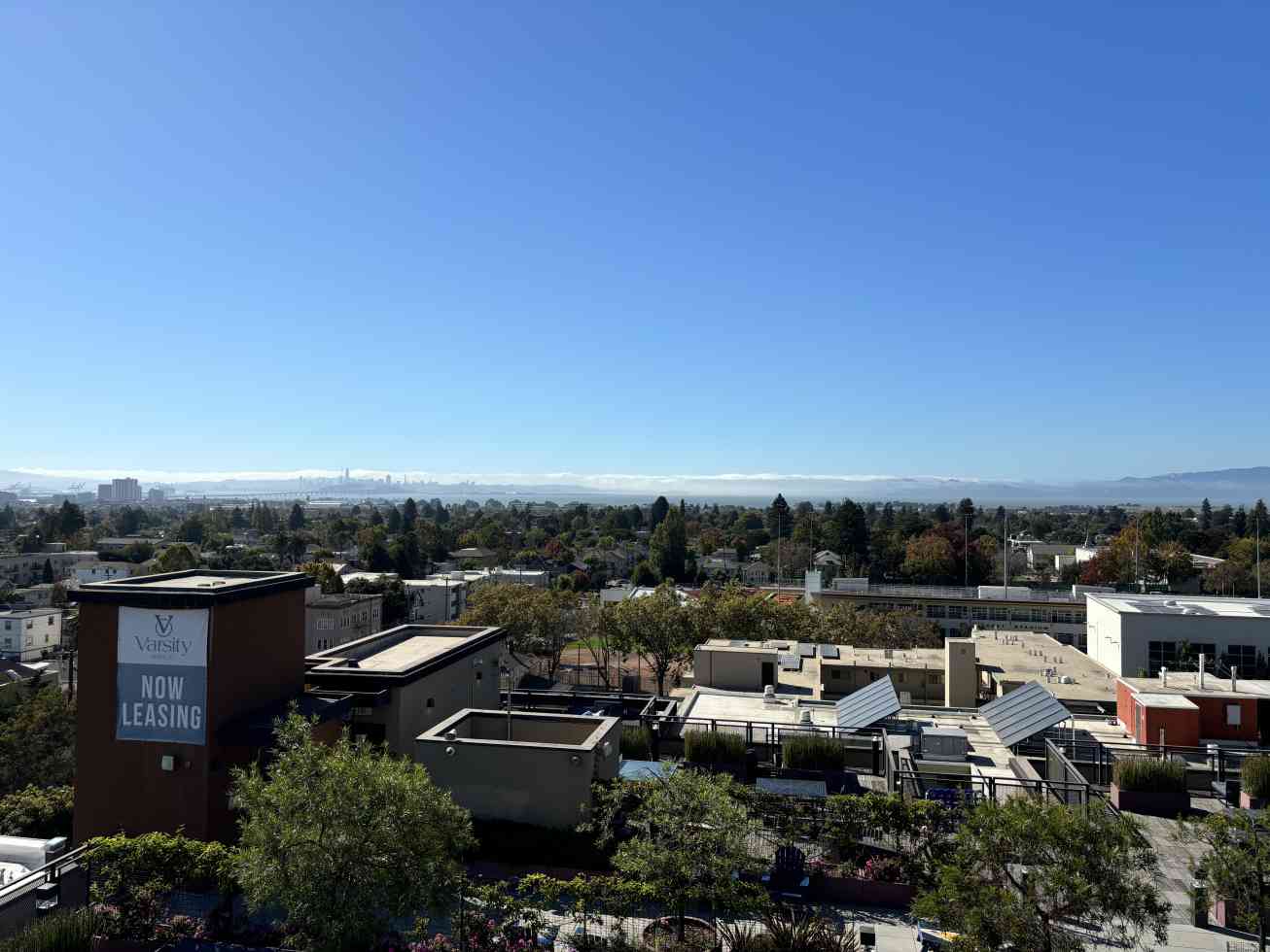
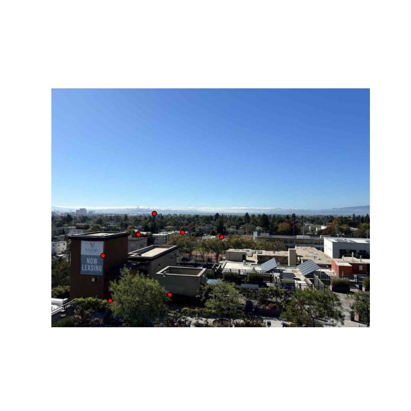
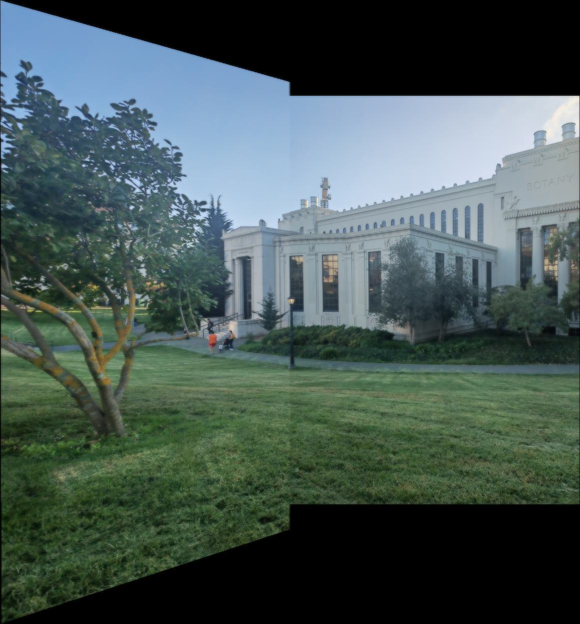
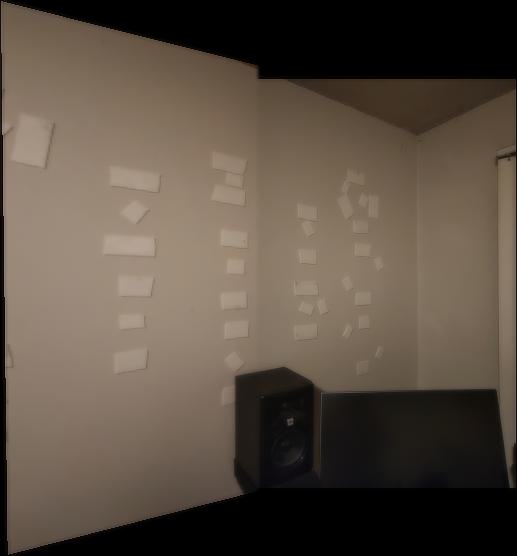
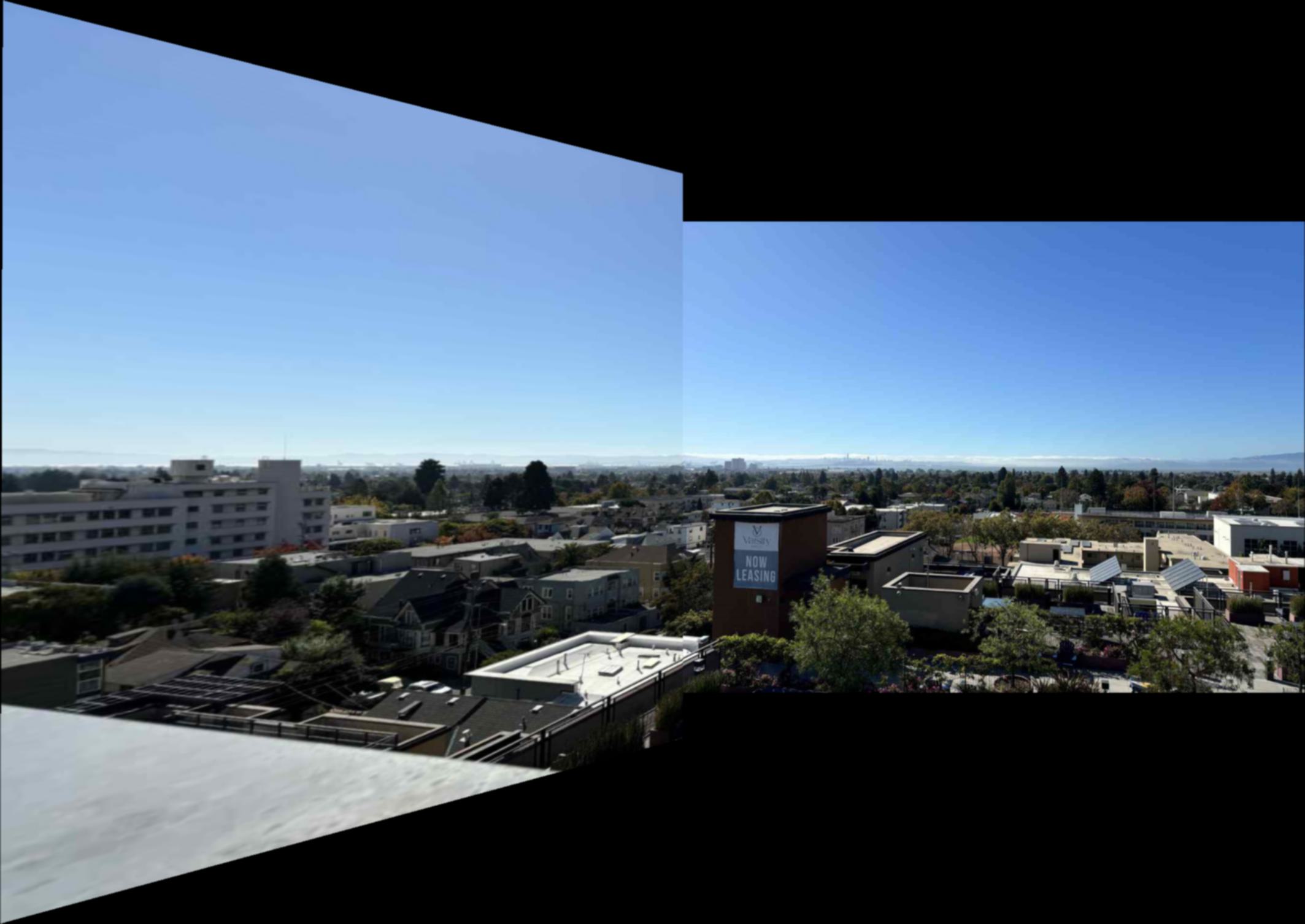
I took some photos from my daily life, which contains my room and some Berkeley views. Meanwhile, I gained some photos which were taken by my classmates. After taking the photo, I utilized the tool given by project 3 to establish the points pairs which help me to calculate homography matrixs.
Calculate Homography
I write a compute_homography function calculates a Homography Matrix between two images, a transformation that allows for perspective shifts, widely used in tasks like image alignment, stereoscopy, and augmented reality within the field of computer vision. The function first ensures that both sets of input points are equal in number and contain at least four points, as these are the prerequisites for computing a homography. It then normalizes these points to boost numerical stability and reduce errors due to scale differences. An equation system, derived from the normalized points, articulates the linear relations that the points must satisfy before and after the transformation. Singular Value Decomposition (SVD) is used to solve this system, effectively handling noise and numerical issues in the data, ensuring an optimal solution even under imperfect conditions. Finally, the computed homography matrix is transformed back to the original coordinate system through a denormalization process.
Image Warp
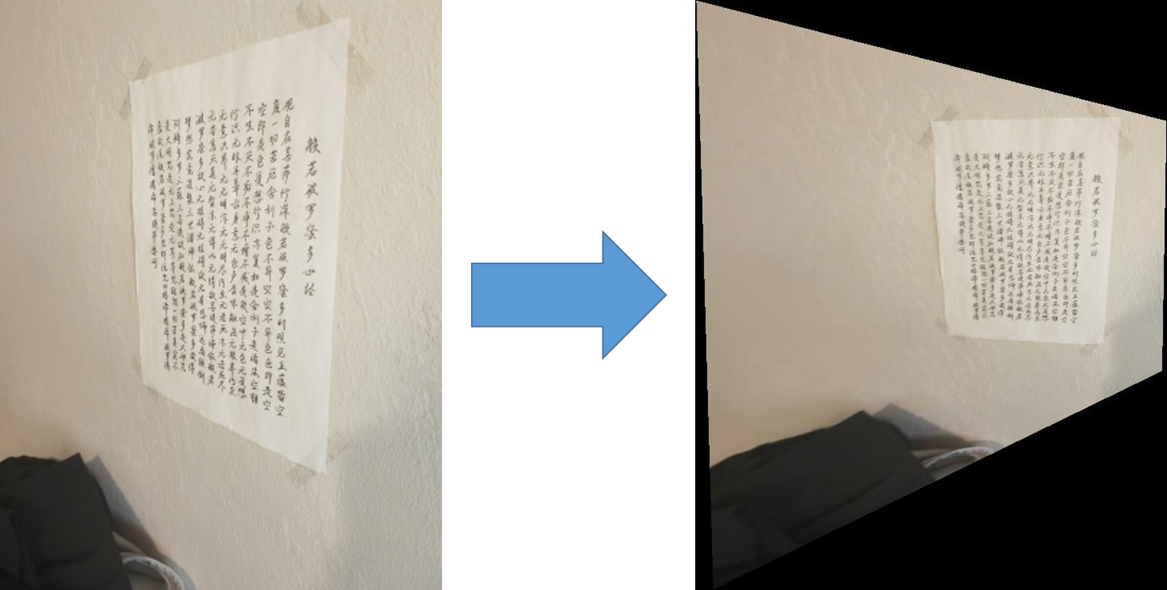
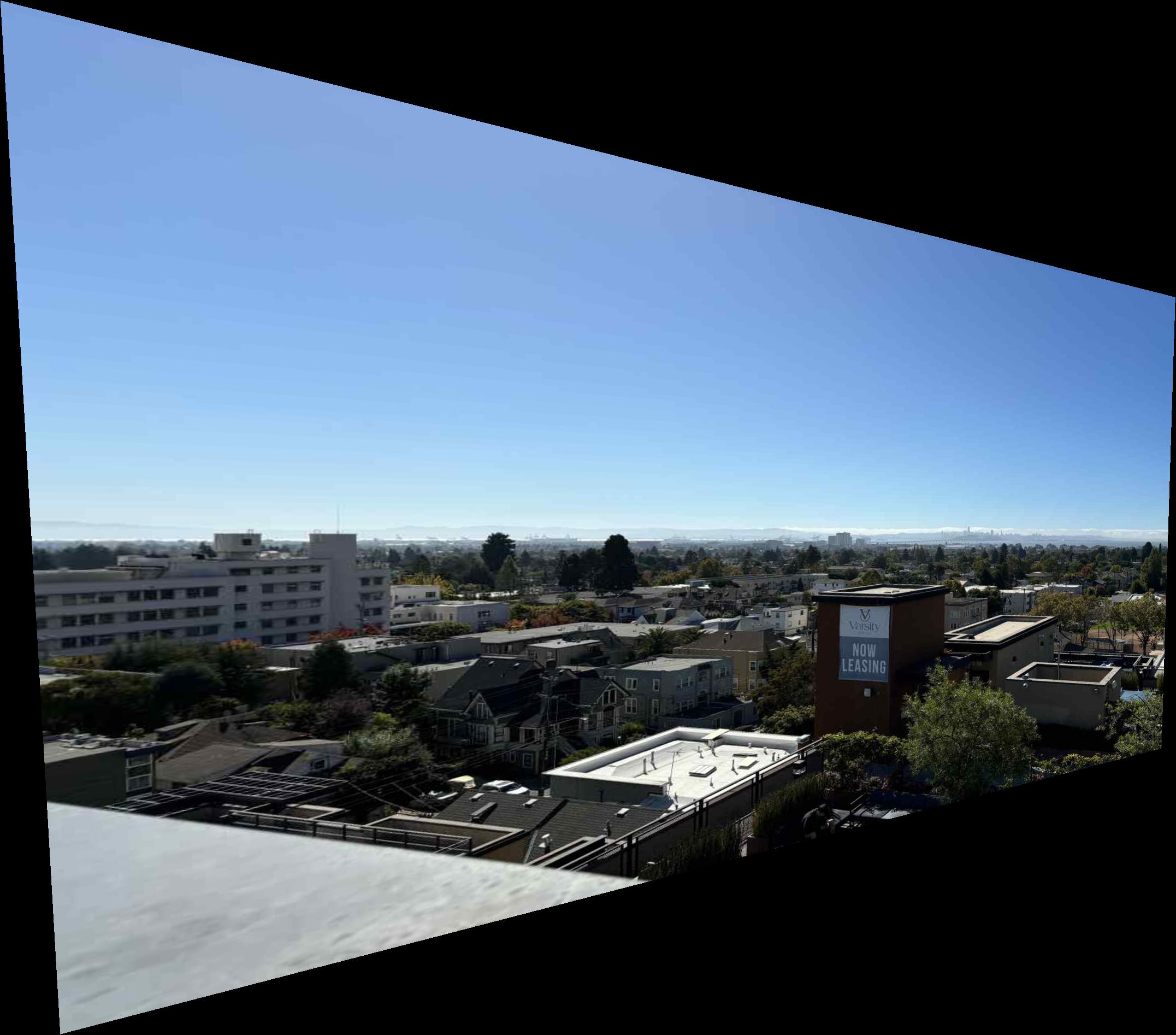
The warpImage function performs a perspective transformation of images using a homography matrix, commonly used in computer vision for tasks like image stitching and perspective correction. Initially, the function determines the dimensions of the image and computes the coordinates of its four corners, converting these into homogeneous coordinates. Using the homography matrix, it transforms these coordinates to new positions and converts the transformed coordinates back to a two-dimensional format. Based on these transformed coordinates, the function defines the boundaries of the transformed image and creates a new coordinate grid that covers the entire transformed area. By inverting the homography matrix, it locates the corresponding positions in the original image for each point on the grid and calculates the pixel values at these positions using interpolation methods, ultimately generating the transformed image. This process ensures the continuity and integrity of the image content while maintaining the quality and visual effects of the transformation through precise interpolation.4
Image Blending
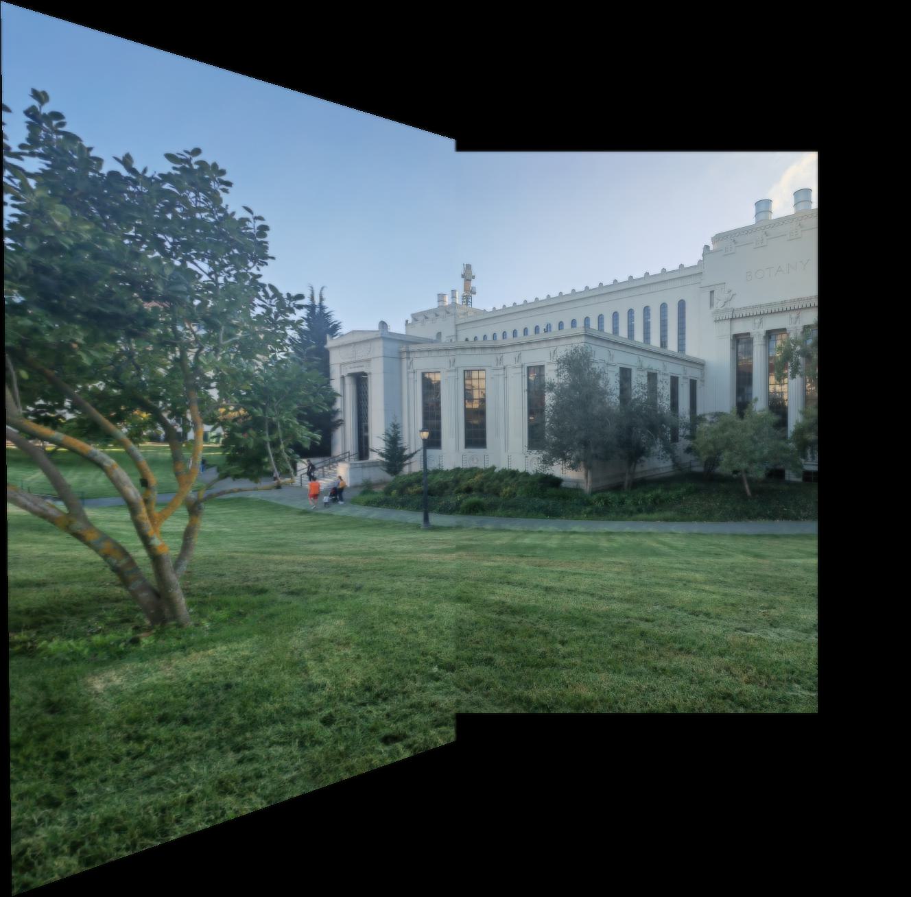
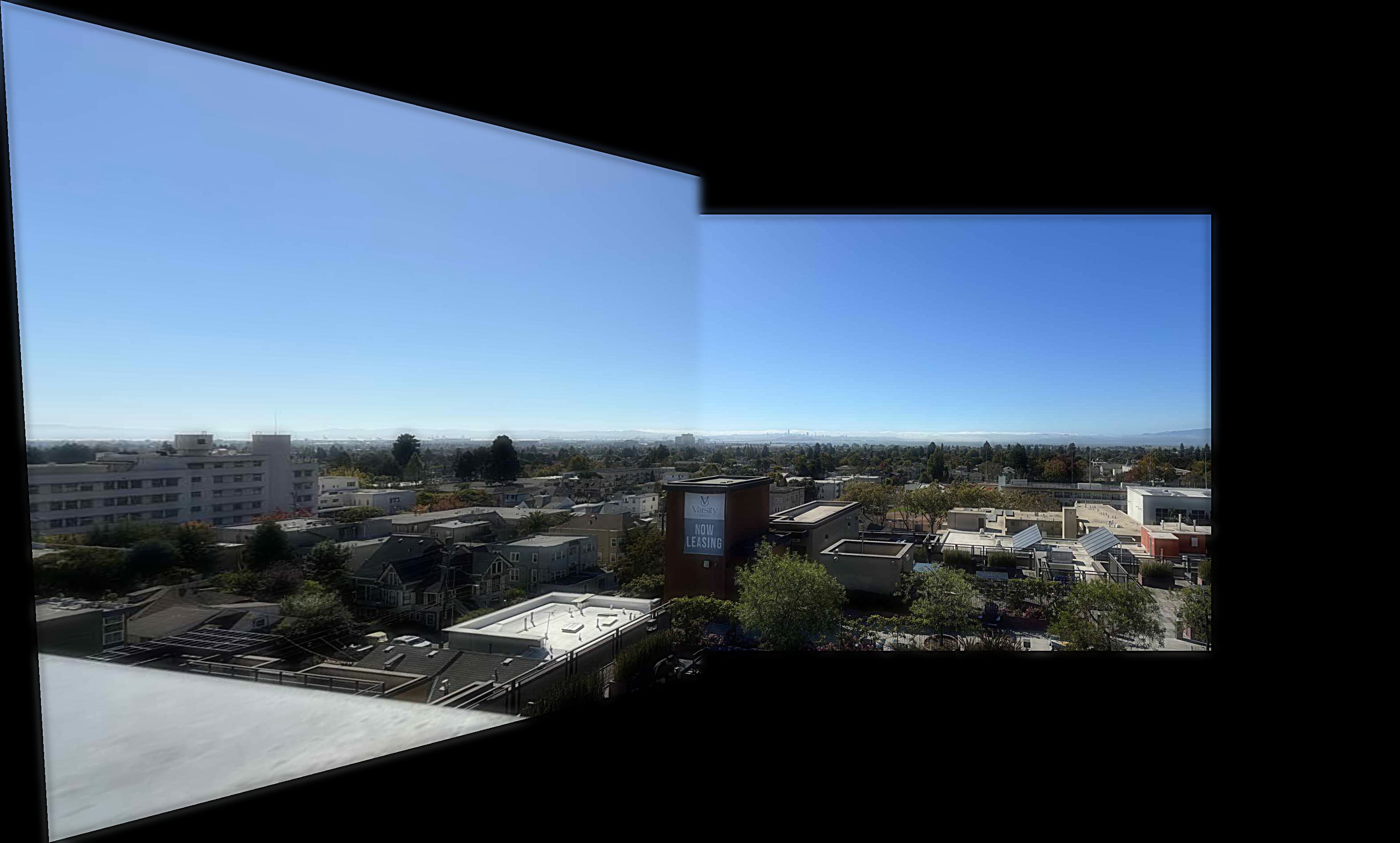
The blend_image function is designed to achieve a smooth blend between two images in a specified overlapping area. This function is typically used in scenarios such as image stitching, where two images partially overlap and a seamless transition is desired.
The function begins by defining an internal function pad_image_to_target which is used to resize images to a specified target size by adding padding to adjust the image position. This ensures that both images align properly for the blending process.
The main blend_image function takes two images image1 and image2, an overlap_ratio that specifies the proportion of the overlap, an offset to adjust the position, and a direction parameter (default "w" for west, indicating a horizontal left-to-right direction). It first calculates the target dimensions to which both images need to be extended so they can be processed on the same canvas.
Next, the function uses pad_image_to_target to pad and position both images appropriately. Depending on the specified direction, the function computes the width of the blend area and the dimensions of the new canvas.
A blending mask mask is then created, which transitions from 0 (black, representing full use of image1) to 1 (white, representing full use of image2) across the blending area. The actual blending is carried out using the Laplacian pyramid technique, which handles image details better, creating a visually natural blending effect.
Finally, the image_blend function performs multi-level blending using Laplacian and Gaussian pyramids to ensure that every detail level transitions smoothly from coarse to fine. Through this method, the function ultimately returns a blended image that visually creates a smooth transition in the overlapping section of the two original images.4


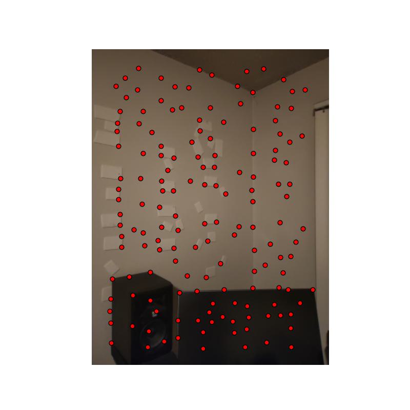
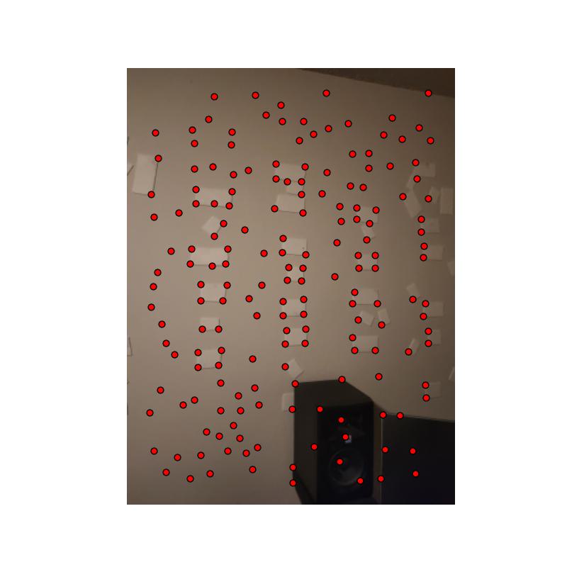
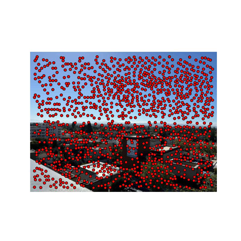
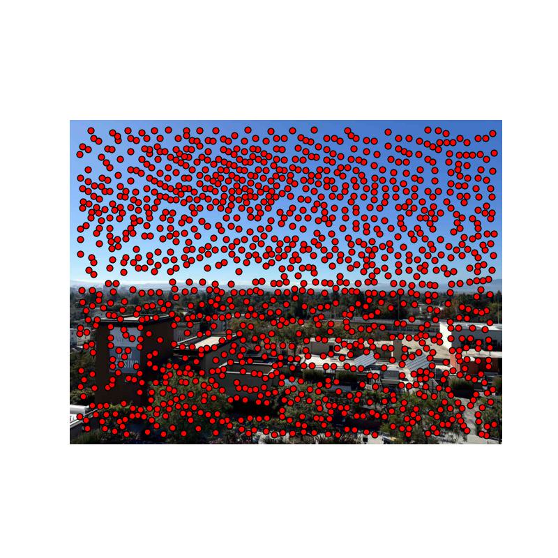
Detecting corner features
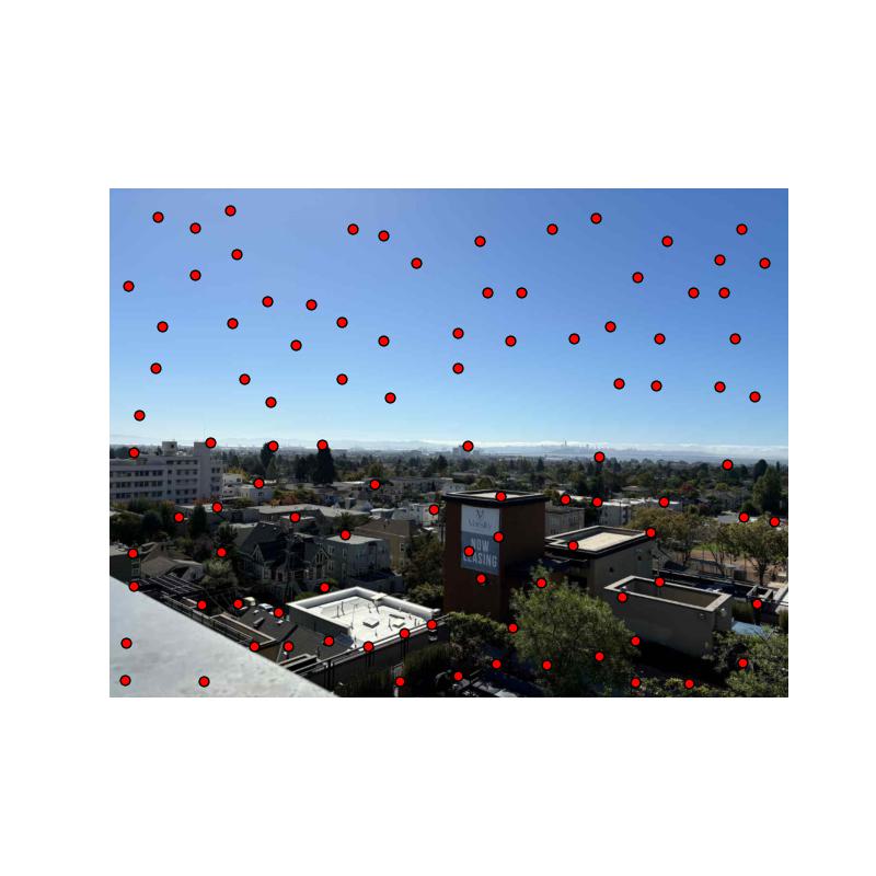
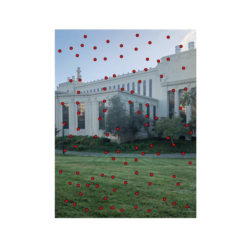
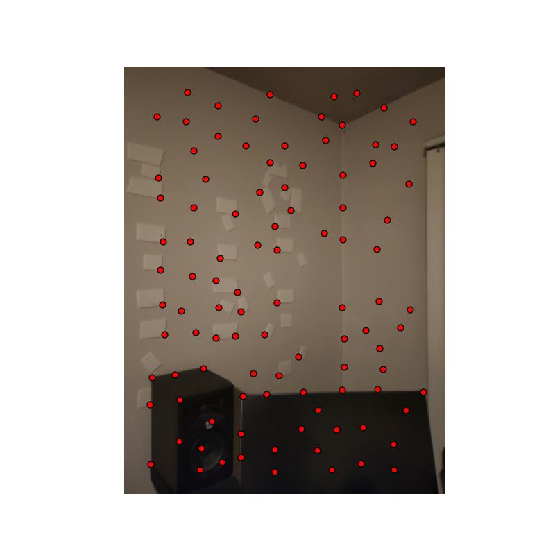
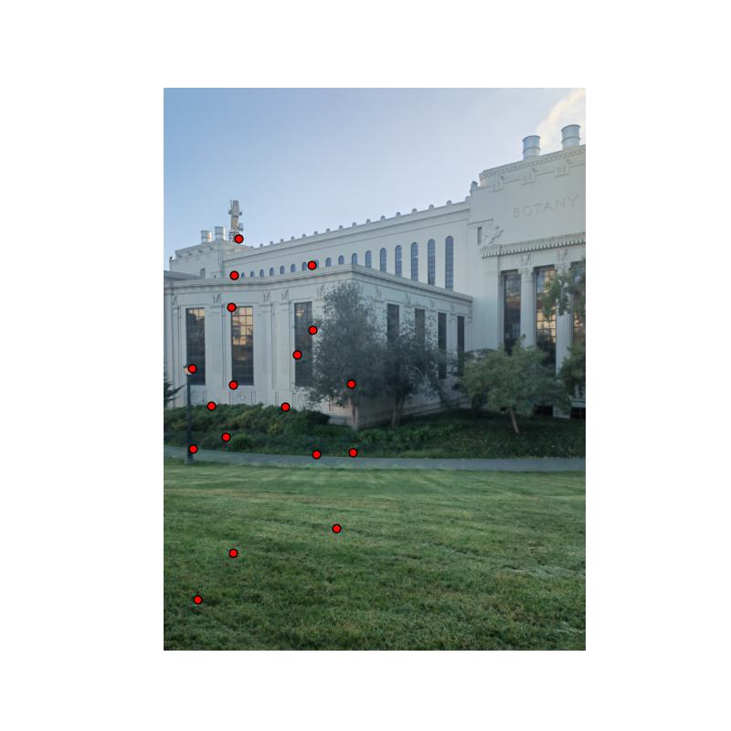
I utilized the function that provided on the website to detect the corner features. Here is the visualization of this part.
Firstly, I input an image, a set of coordinates, and two window size parameters: a larger window (large_window) and a smaller central window (small_window). To facilitate the processing of coordinates at the image edges, the original image is initially padded around the edges with a width equal to half of the large window, using a padding value of 0. For each coordinate, the function extracts a large window region centered around the point from the padded image, then further extracts a smaller window area from the center of this region. This smaller area's pixel values are normalized (by subtracting the mean and dividing by the standard deviation) only if the standard deviation of this area is greater than zero, and the processed data is flattened into a one-dimensional array to serve as a descriptor. All these descriptors are eventually stored and returned as a NumPy array.
Feature Descriptors
Match Descriptors
Adaptive Non-maximal Suppression
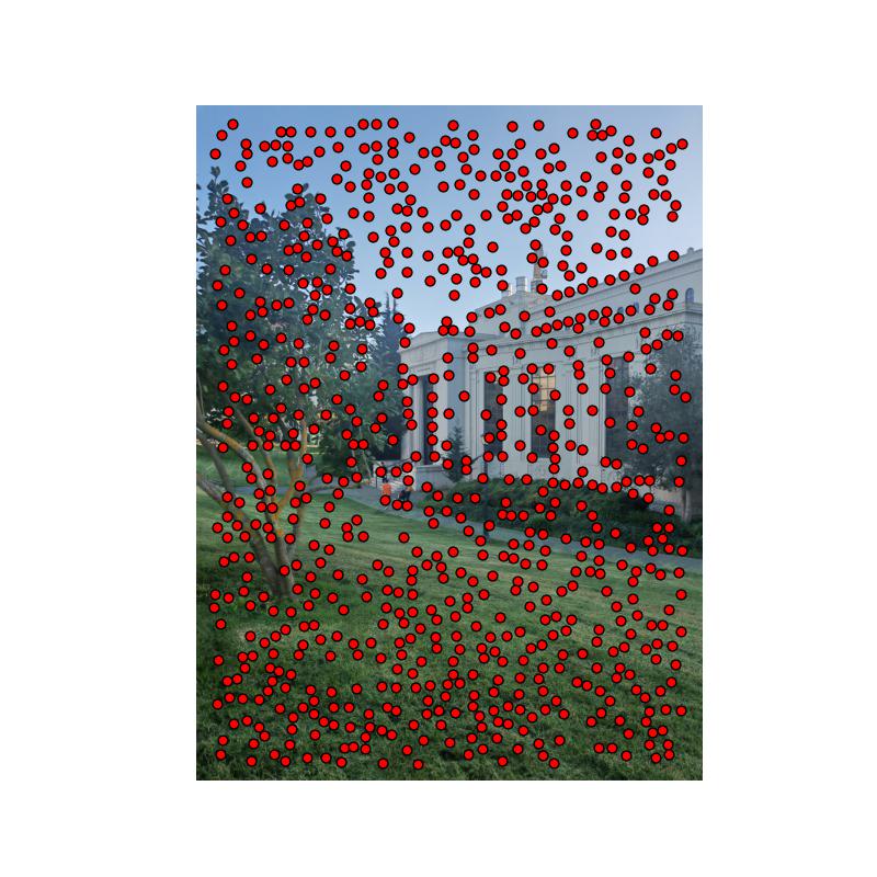
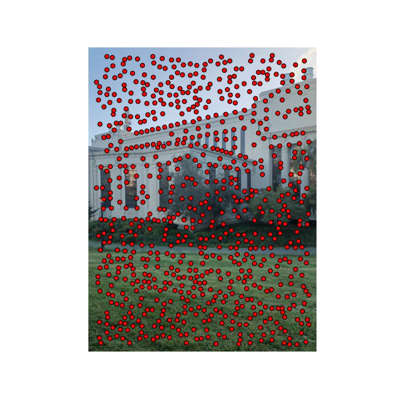
First, I input a set of coordinates coords, an image's keypoint response matrix h, and an optional parameter for the number of points num_points. The function initializes an infinite distance array radii, and for each point, it calculates and updates the minimum distance to other points with higher response values. Then, it sorts these distances in descending order and selects the top num_points with the largest distances, returning their coordinates. This method reduces the number of keypoints, thereby lightening the computational load for subsequent processing while retaining the points most likely to represent significant features. It is particularly well-suited for tasks involving image matching and recognition. (This block I refered to several websites and paper such as CSDN and Github). Here is the result.


I use squared Euclidean distance to calculate the similarity between descriptors, and apply Lowe's ratio test to enhance the reliability of the matches. The function first iterates through each descriptor in the first set, descriptors1, computing the squared Euclidean distance to all descriptors in the second set, descriptors2. It then identifies the two closest points for each descriptor. If the closest distance is less than a set ratio (defaulted to 0.75 times) of the second closest distance, the pair of descriptors is considered a valid match and their indices are added to the match list.
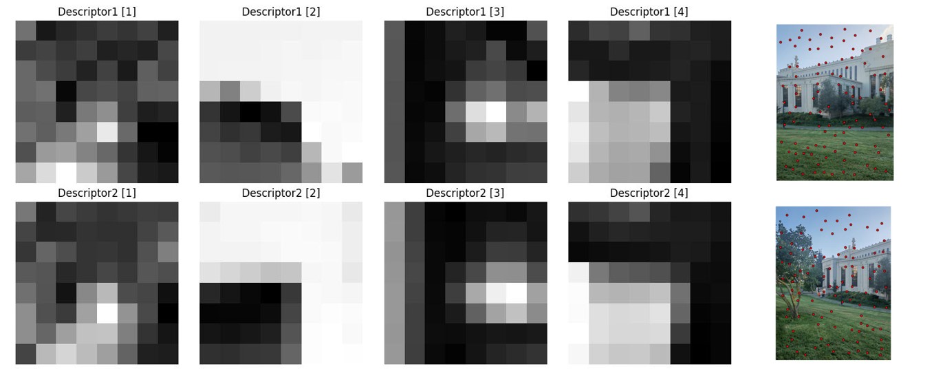
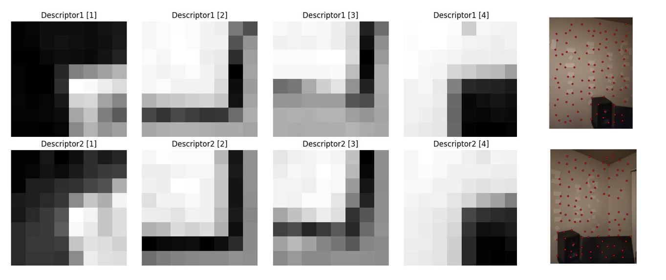
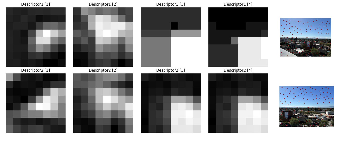
Here are some paired descriptors in different images.
RANSAC
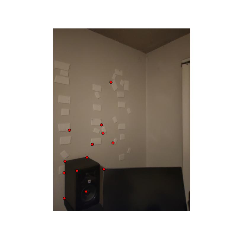
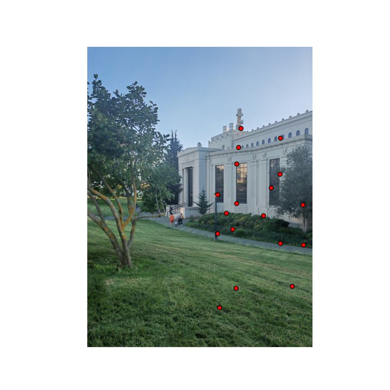
I start by initializing the maximum number of inliers, the best homography matrix, and the list of inliers. Within the set number of iterations, each iteration randomly selects four pairs of source and destination points, computes the homography matrix, and transforms all source points according to this matrix. Afterwards, I calculate the distance between the transformed points and the destination points, and determine which points have errors within the threshold, marking them as inliers. If the number of inliers from the current iteration exceeds the previous record, then the best homography matrix and its list of inliers are updated. Finally, the function returns the homography matrix and list of inliers that had the most inliers found during the iterative process. Here are the result which shows the inliner points.
After selected the best inliner points, I recalculated the homography matrix to get a better result.
Lorem ipsum dolor sit amet, consectetur adipiscing elit. Suspendisse varius enim in eros elementum tristique. Duis cursus, mi quis viverra ornare, eros dolor interdum nulla, ut commodo diam libero vitae erat. Aenean faucibus nibh et justo cursus id rutrum lorem imperdiet. Nunc ut sem vitae risus tristique posuere.
Blend Comparison
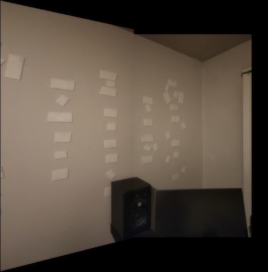
Left side is the manual blend images and right side is the auto blend images
